
Introduction
Robust underwriting is a key element of any commercial real estate (CRE) investor’s success. Currently, institutional and retail CRE investors typically employ some form of static discounted cash flow (DCF) modelling to value properties and identify attractive investments. Unfortunately, static DCF modelling suffers from several flaws that stem from its inability to take uncertainty into account. While investors frequently employ some form of sensitivity analysis by using various upside and downside cases, this method does not consider the full range of potential outcomes, or the probability of each outcome occurring, and may lead to suboptimal decision making. However, Monte Carlo Simulation (MCS) methods that are easy to implement and are presently used to value various other financial instruments like options and mortgage-backed securities, can improve underwriting robustness and improve decision making. MCS uses a probability distribution to randomize various uncertain inputs. For example, we might use the normal distribution, or “bell curve” to model inputs like rental growth rates. We would use estimates of the mean and standard deviation of this growth rate based on historical data as inputs to the normal distribution. The resulting outputs are then recorded as this process is repeated hundreds or even thousands of times, culminating in a distribution of outputs.
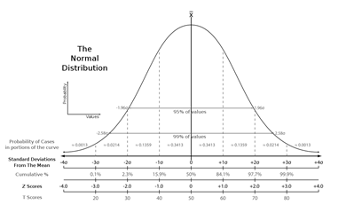 Figure 1: The Normal Distribution
Trillions of dollars are on the line in CRE transactions each year, so some investors might be hesitant to employ a new valuation technique if they do not fully understand it. However, the amount of capital on the line is an even better reason to employ more sophisticated valuation techniques. The advantages and rationale of MCS methods will be further illustrated below using an example.
Rationale
An MIT research paper by Keith Chin-Kee Leung illustrated the value of using a simple MCS model over a static DCF. Consider a 10-story office building with 17,000 sq ft floor plates. The simple model used a classic static DCF with a 3% rental growth rate over a ten-year period. A second model randomizes the rental growth rate using a normal distribution. The second model uses the same 3% average growth rate and a 2% standard deviation to parameterize the probability distribution. These two models should come up with the same ENPV since they use the same average growth rate, right? Wrong. In fact, the ENPV for the MCS model was more than $500,000 more than the static model. This is a substantial variation and could be the difference between winning a bid or not. But what are the reasons the MCS model consistently produces a higher NPV compared to the static DCF model despite using the same average growth rates?
The answer lies in the nonlinearity of the model and is explained by the Flaw of Averages and Jensen’s Inequality, which states that outputs from a non-linear function will generally not equal the output obtained by using the average value of the input parameters. Put more simply, since ADR growth is compounded (nonlinear) the average output in a MCS does not equal the NPV found using the same mean. To illustrate, consider a property with revenue of $1 million in year 1 which grows by 3% for 10 years to $1.344 million. If instead we use two iterations of the MCS output with growth rates of 2% and 4% resulting in NPVs of $1.219 million and $1.480 million respectively, we find that the average NPV comes out to $1.35 million –despite the same 3% average growth rate between the two scenarios. Thinking about this in another way, in the low growth scenario the revenue was only $125,000 less than the base case, while in the high growth case the revenue is $136,000 more. This also illustrates the fact that the more compounding periods that occur, the greater this effect will be. Of course, there are many other inputs to a property valuation model where these non-linearities exist and the model would be biased if the only dynamic input pertained to revenue growth.
 Figure 2: Illustrating the Flaw of Averages
Now that some of the advantages and rationale of MCS have been outlined, other applications of MCS will be further illustrated.
Risk Management Applications
A truly robust model would apply MCS to all uncertain inputs in a model including occupancy rates, expense growth rates, capital expenditure growth rates, discount rates if floating rate debt is used, cap rates, and more. For expenditures, the Flaw of Averages would work in reverse and expected expenses would be higher than in a static model. As more sources of uncertainty are added to the model, more volatility will be introduced and the better the full range of outcomes of an investment can be understood. As was illustrated by the office tower example, an MCS model could come to a substantially different valuation than a static one, but a potentially greater aspect of MCS is the ability to analyze the entire distribution of outcomes.
If a fund measures performance using IRR, for example, the probability of exceeding the fund target can be calculated by dividing the number of MCS iterations that exceed the IRR target by the total number of iterations. This concept can be further expanded to determine the probability of losing money or to calculate how severe losses will be in the case of a negative NPV investment. More sophisticated measures like value at risk (VaR)—a measure frequently used by banks and other financial institutions—can be used to measure losses in very low probability events. VaR measures the severity of losses over a set time-period with a given probability. For example, if a CRE portfolio has a one year 5% VaR of $1 million, it means that there is a 5% chance that this portfolio will decrease in value by $1 million. An alternative interpretation is that this portfolio should be expected to lose $1 million in 1 out of every 20 years (due to the 5% probability).
Overall, there are a great number of tools that can be used to fully understand the risk profile of an investment. However, how can a MCS model, and the aforementioned risk and return metrics, be easily calculated? The implementation will now be discussed using an example that was executed exclusively using Microsoft Excel and built-in functions with no add-ons or supporting software.
Example & Execution
Executing a Monte Carlo Simulation in Excel
Consider a 150 key, New York City hotel property, with average daily rate (ADR) growth being the only probabilistic or non-static input. Say that it is know that the historic ADR growth rate for this type of property averages 3% per year with a standard deviation of 2%, and that the distribution of growth rates is known to resemble a bell curve, or a normal distribution. The model generates a random probability using Rand() which generates a random decimal between zero and one. This probability becomes an input to the Norm.Inv() function alongside the 3% mean and 2% standard deviation. The function that outputs the random growth rate for this case will appear as =Norm.Inv(Rand(), 3% , 2%) or generically as =Norm.Inv(Rand(), [mean] , [standard deviation]). However, this only generates a single random case and not the hundreds or thousands of iterations required for an MCS.
This can be achieved easily using Excel’s data table functionality. A column of iteration numbers, in this case 1 to 1,000 is recorded in column A, rows 2 through 2,000. In cell B2, the NPV based upon the current case’s inputs is referenced. Creating a data table using any blank cell as the column input cell will generate a table of 1,000 NPVs based on 1,000 randomly generated ADR growth rates. Summary statistics can now be taken (ENPV, standard deviation, range, etc.) to assist in better understand the risk profile of the property relative to a single NPV or several NPVs based on baseline, downside, and upside cases.
Adding Complexity to the Model
Since making ADR growth the only randomized input will bias the model to the upside, the model will now be expanded to include dynamic occupancy growth, expense growth, exit cap rate as well as ADR growth. (See figure 3 for a summary of distribution parameters.) For simplicity, the normal distribution is again used for each of these inputs. As can be seen in figure 4, the fully dynamic model has a significantly higher standard deviation at $2.6 million compared to the $1.5 million in the model with dynamic ADR growth alone. Furthermore, the range of outcomes is 44% wider at $17.4 million between the highest and lowest outcomes. (See figure 4 for the full comparison of summary statistics between models.) This information is partially lost in a static model, even if a scenario analysis is conducted because no standard deviation can be calculated, and it is unclear what the likelihood of any given outcome is. However, this is not the case in MCS as we can display the full probability distribution using a histogram.
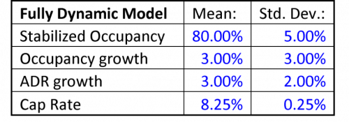 Figure 3: Summary of Distribution Parameters
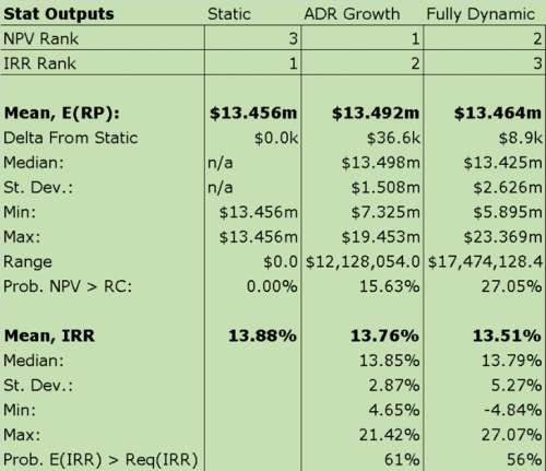 Figure 4: Summary Statistic Comparison
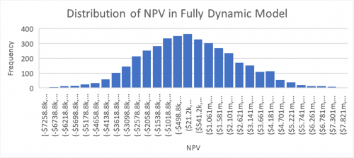 Figure 5: Fully Dynamic Model NPV Distribution
Overall, there are a great number of tools that can be used to fully understand the risk profile of an investment. While these tools can be extremely helpful, they still suffer from the old adage “garbage in, garbage out”, so is the assumption of a normal distribution reasonable?
Garbage in Garbage Out
As mentioned, an MCS model is only as good as the assumptions that go into it. As more granular data on real estate parameters and performance becomes available, models should be able to better incorporate historic trends alongside the intuition and experience of industry experts. For the purposes of this piece, the distribution of revenue growth will be proxied by public and private CRE performance.
Since expenses are less likely to exhibit significant volatility relative to revenue, it makes some sense to proxy the distribution by CRE returns starting with NAREIT index returns. As seen in Figure 6, the quantile-quantile plot of returns is plotted against a normal distribution parameterized by the mean and standard deviation of returns. A quantile-quantile plot graphs the actual percentile of a data point relative to the rest of the data versus the theoretical quantile that would be expected if the data were normally distributed. Therefore, if the returns are normally distributed, the points should lie along the red line of the Q-Q plot. This relationship holds well for the middle portion of the distribution but fails for very high and very low returns. This is because the true distribution is “fat-tailed” or “heavy-tailed”. This means that has a greater portion of the probability distribution is contained in the extremes of the distribution relative to the normal distribution. (See figure 7 for an illustration of heavy tails.)
The fatness of tails can be measured using the fourth moment or kurtosis. NAREIT index returns display a Kurtosis of 10.3 which means that the distribution has fatter tails than would be expected from a normal distribution (Kurtosis of 0 indicates that the tails contain the same portion of the distribution as the normal distribution.) Furthermore, the true distribution is negatively skewed (relative to the normal distribution, more of the distribution is contained in the extremely low outcomes), so using a normal distribution to model revenue may result in an optimistic forecast relative to the true distribution.
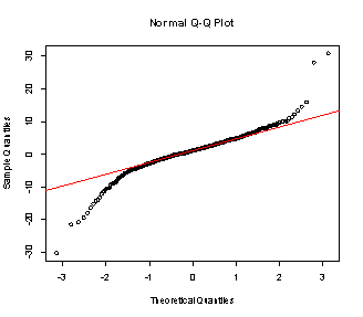 Figure 6: Q-Q Plot of NAREIT Returns
Skew: -.4789385
Kurtosis: 10.31126
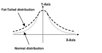 Figure 7: Illustration of a Fat-Tailed Distribution
Due to the publicly traded nature of REITs, this performance may vary from private CRE performance. However, conducting the same analysis on NCREIF Property Index returns reveals a similar phenomenon. In this case, the tails of the distribution are less fat than in the publicly traded REIT performance. This may be because of reduced liquidity, and therefore the limited ability of investors to sell when things are bad or buy when they are good. However, the skew is even more negative at -1.45. This means that the normal distribution would be even more optimistic relative to reality.
All this goes to show that while MCS can be a powerful tool for valuation and risk management, it is susceptible to poor assumptions and investors must be careful to properly parameterize their models. Furthermore, historic performance is not always indicative of future performance, so things like market cyclicality, volatility regimes, and momentum should also be applied to models to most accurately value properties.
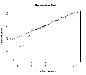 Figure 8: Q-Q Plot of NPI Returns
Skew: -1.452594
Kurtosis: 5.676668
Conclusion
As was illustrated, the mathematical rationale for using MCS is strong. The Flaw of Averages leads static models to over or under-value properties by significant amounts due to non-linearity and may be the difference between winning or losing a bid. In addition to more accurate underwriting, MCS can be used in a variety of risk and return management applications including calculating probability of hitting return targets, computing expected gains, losses, and VaR, measuring variability and helping to visualize return distributions. However, MCS driven models are only as good as their input assumptions, so investors must be careful to parameterize their distributions accurately by analyzing historic data while overlaying their industry expertise to account for changes in the market. When executed correctly, MCS is a powerful tool that can be implemented with relative ease. Real Estate investors should consider adding this tool to their toolbox as has been done in many other areas of finance and investments.
